The True Story
Maya had one month to turn a season of farm imagery into something her client could act on. The brief sounded clean in the kickoff meeting: segment crop boundaries, detect stress patterns, compare model families, and return maps that the agronomy team could trust. In the notebook, it became messier. The same farm looked different after the rain. A boundary that was obvious in one tile faded into bare soil in another. Some labels were beautifully drawn; others carried the small compromises of field work. She was not training one model so much as trying to make three different ways of seeing agree with one another.
The first model was a U-Net for crop boundary segmentation. The second was a more targeted segmentation pipeline for stressed canopy, bare soil, and broken rows. The third was a ViT experiment, included because she suspected a transformer might notice field-level patterns that the convolutional models missed. None of those experiments was exotic on its own. The problem was the calendar. A month is a long time when a team is making slides; it is a short time when every training run waits behind preprocessing, every validation pass competes for GPU time, and every mistake costs another night.
Her company had bought GPU credits for the project, and she felt their weight every time she launched a run. Use too small a machine and the training crawled. Use too large a GPU for a preprocessing job and the budget burned for no reason. Run everything sequentially and the month disappeared. Run everything manually and she spent half the day hunting job ids, logs, and half-failed outputs. The work was not impossible, but it was narrow: one month, several models, one shared pile of imagery, and no room for a week of infrastructure setup.
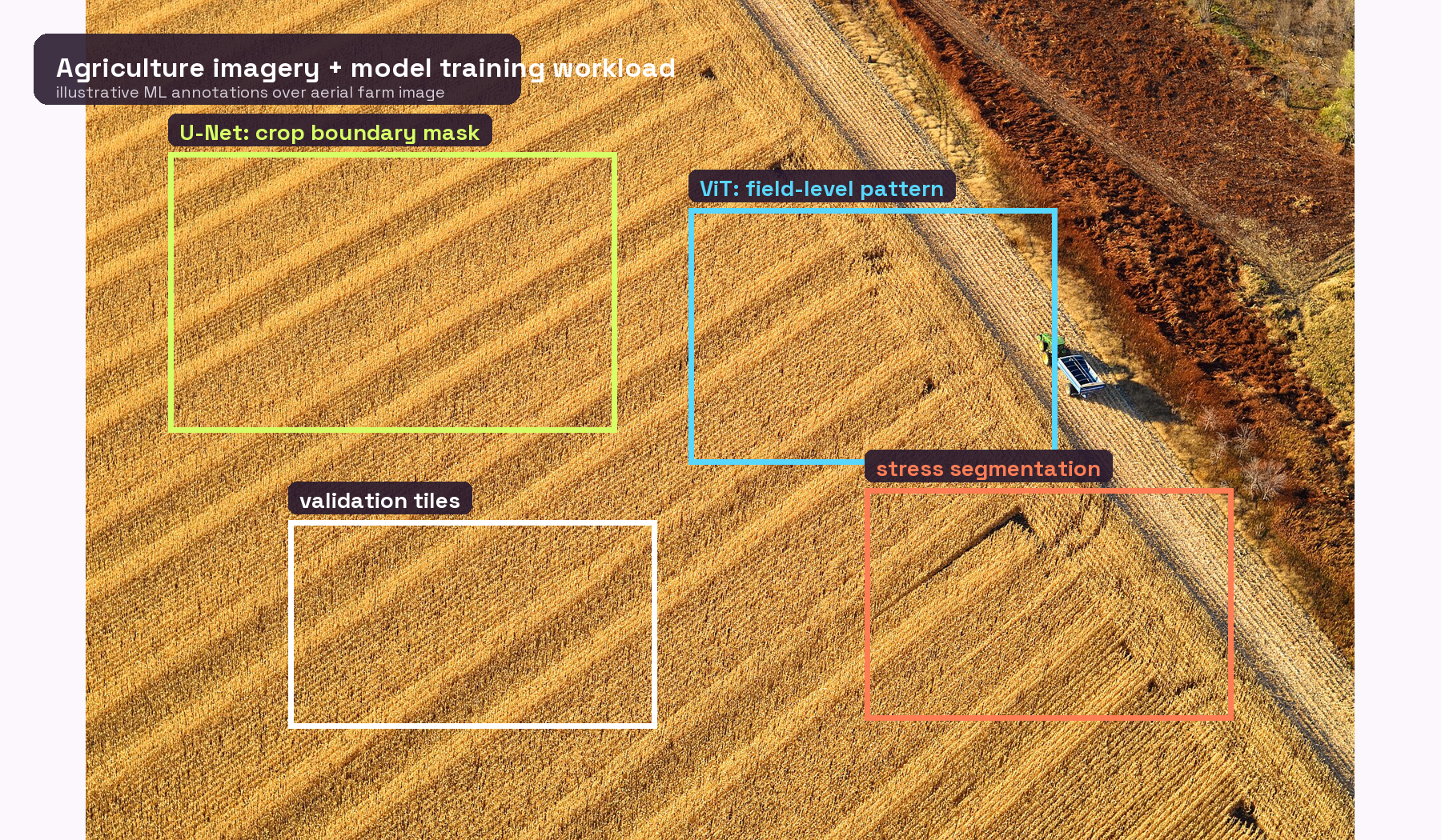
Illustrative ML annotations over aerial farm imagery. Source image: South Dakota Farm Corn Harvest Aerial 4, Carl Young, Wikimedia Commons, CC BY-SA 4.0; annotations added for this draft
The first try: Dask
Dask was the natural first stop because Maya already thought in arrays and batches. It made sense for fanning out preprocessing: split the imagery, clip the tiles, build masks, and let workers chew through the queue. For that slice of the project, Dask felt honest and useful.
But Dask did not remove the rest of the work. She still needed to configure or borrow a cluster, choose worker sizes, watch memory pressure, keep GDAL and rasterio aligned, wire storage, capture logs, and recover when one worker died on a tile with a huge geometry. It helped her parallelize Python; it did not become the geospatial workbench around the project.
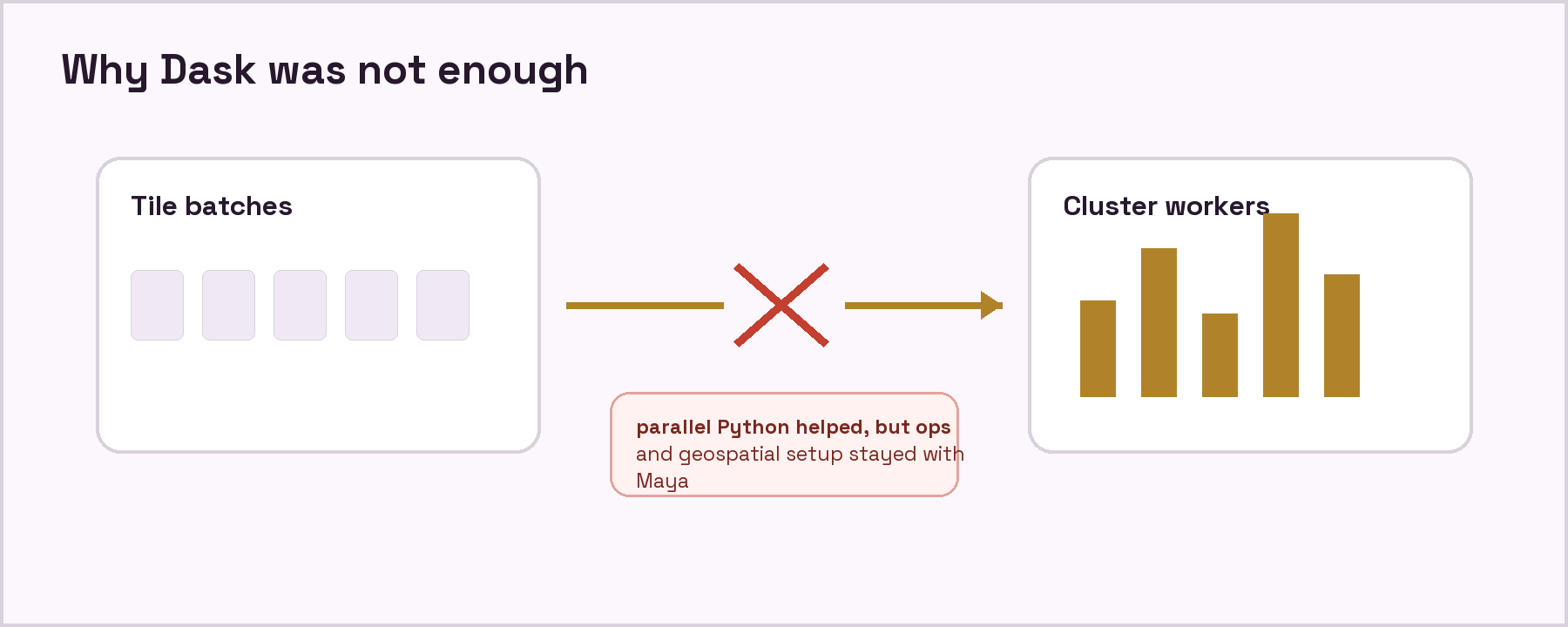
Illustration: Dask handled distributed work, but the project still needed cluster operations, storage wiring, and geospatial dependency control.
The second try: Tuner
Tuner came next because part of the job really did look like model experimentation. Maya needed to compare encoders, learning rates, checkpoints, and validation curves. A tuning system promised order: run the sweep, collect the metrics, pick the winner.
The problem was that her agriculture project was not only a tuning problem. Some tasks were CPU-heavy. Some needed high RAM. Some needed a T4. A few might justify H100-class training. The outputs also needed to land back beside the imagery, labels, masks, and maps the rest of the team used. Tuner could organize model choices, but it did not solve the shared geospatial storage, mixed compute, annotation, and map-output workflow around those choices.
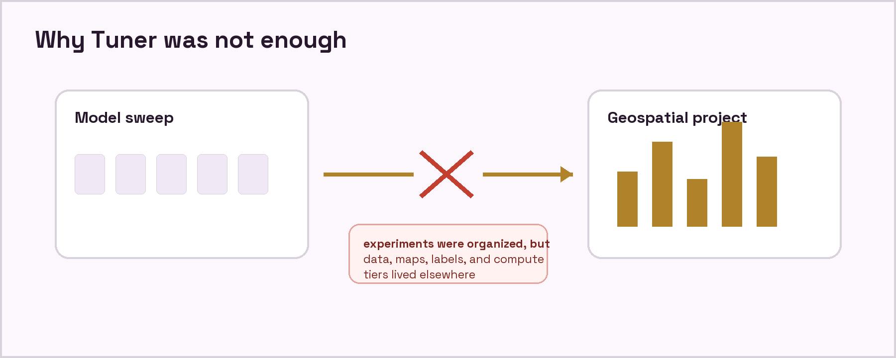
Illustration: the model-sweep layer was useful, but the agriculture project needed a full geospatial workflow.
The third try: Modal, the closest miss
Modal was the closest thing to what she wanted. It had many of the right instincts: remote functions, clean developer ergonomics, fast containers, GPU access, secrets, scheduled jobs, queues, and a much friendlier path to cloud execution than building everything from scratch. Maya could imagine putting a training function behind Modal and finally getting out of the cluster business.
But her use case had one hard no: the 24-hour timeout cap per function. Some training runs might finish in six hours; some might not. Some would need to resume, fan out, create child work, or run overnight while she watched usage the next morning. The cap forced her to redesign the model around the platform limit instead of the agriculture workload. Modal was powerful, but it still did not give her a shared geospatial data lake, labeler, map-aware project space, and run UI in the same place.
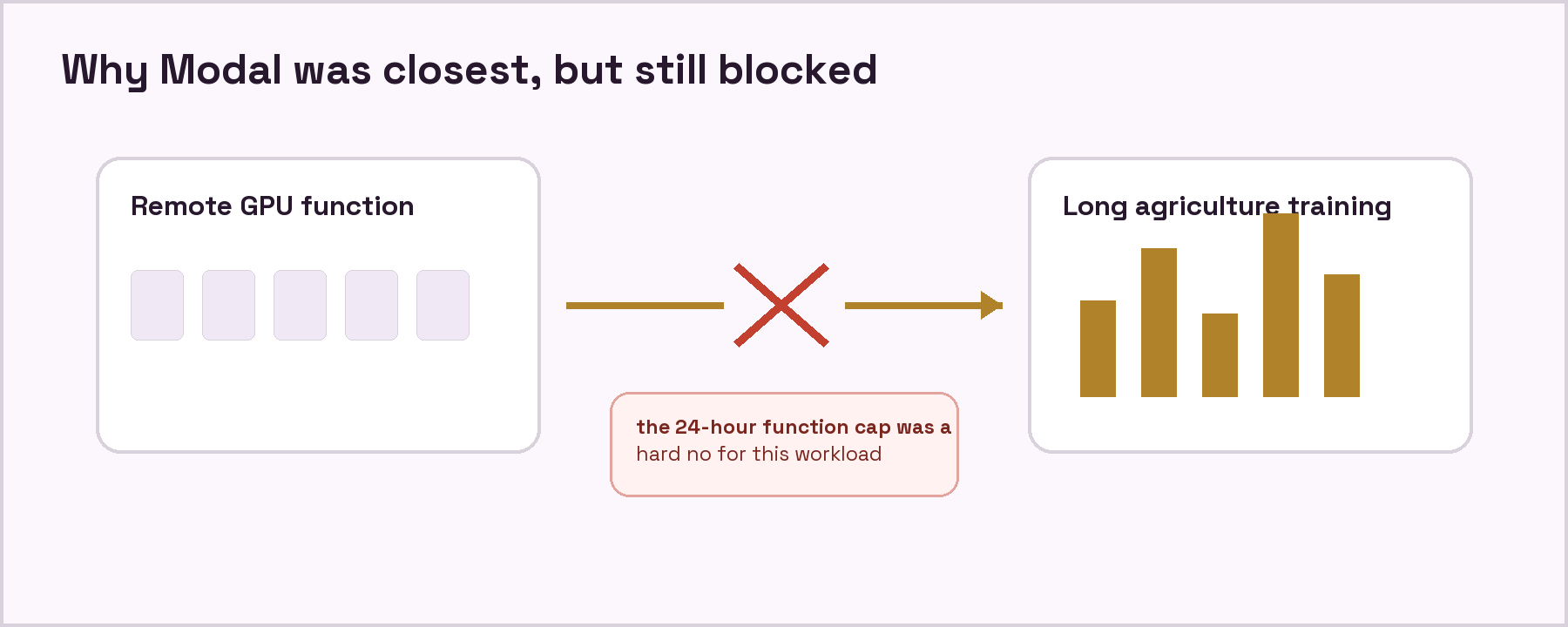
Illustration: Modal came closest technically, but long-running agriculture training could not be designed around a strict function timeout.
What she actually needed
By the second week, Maya could describe all the missing features from all the tools she tested. She needed to run one model across many batches from the same storage, run different model families overnight, choose CPU or GPU by task, and see every job without writing another command just to check whether a run was alive.
Fan out one segmentation model across many image batches from the same shared storage.
Train U-Net, stress segmentation, and ViT experiments at the same time.
Use CPU machines for preprocessing and validation instead of wasting GPU credits.
Use T4 for ordinary training or inference and reserve H100-class compute for runs that justified it.
See status, logs, child runs, elapsed time, CPU/GPU/RAM usage, and failures in one UI.
The Reddit moment
The answer did not arrive as a vendor deck. It arrived the way many practical engineering answers do: in a Reddit thread, buried between GPU pricing complaints and CUDA install stories. Someone mentioned NIKA Runner inside NikaPlanet: a geospatial workbench where a Python function could be decorated with @run, submitted to managed compute with .submit(), and watched from a UI that understood runs, children, logs, and machine usage.
Maya almost dismissed it because most 'simple' tools become complicated the moment the data is real. But NIKA Runner was not floating by itself. It lived inside NikaPlanet, where the same team workspace could hold imagery, labels, masks, notebooks, maps, and shared project storage. That mattered. She did not want a standalone compute island. She needed more compute choices beside the data.
The syntax was small enough to trust
Maya did not have one clean script waiting to be productized. She had about ten notebooks: one for clipping imagery, one for chip generation, one for U-Net training, one for stress segmentation, one for ViT experiments, one for validation, and several small notebooks that only made sense because she had written them at 1 a.m. Rewriting all of that into a new platform would have cost the very week she was trying to save.
That is why the decorator mattered. The first layer was not a new workflow language. It was the smallest possible boundary around code she already trusted: import run, put @run(...) above the function she wanted to offload, and call .submit() when she wanted it to run in the background instead of blocking the notebook.
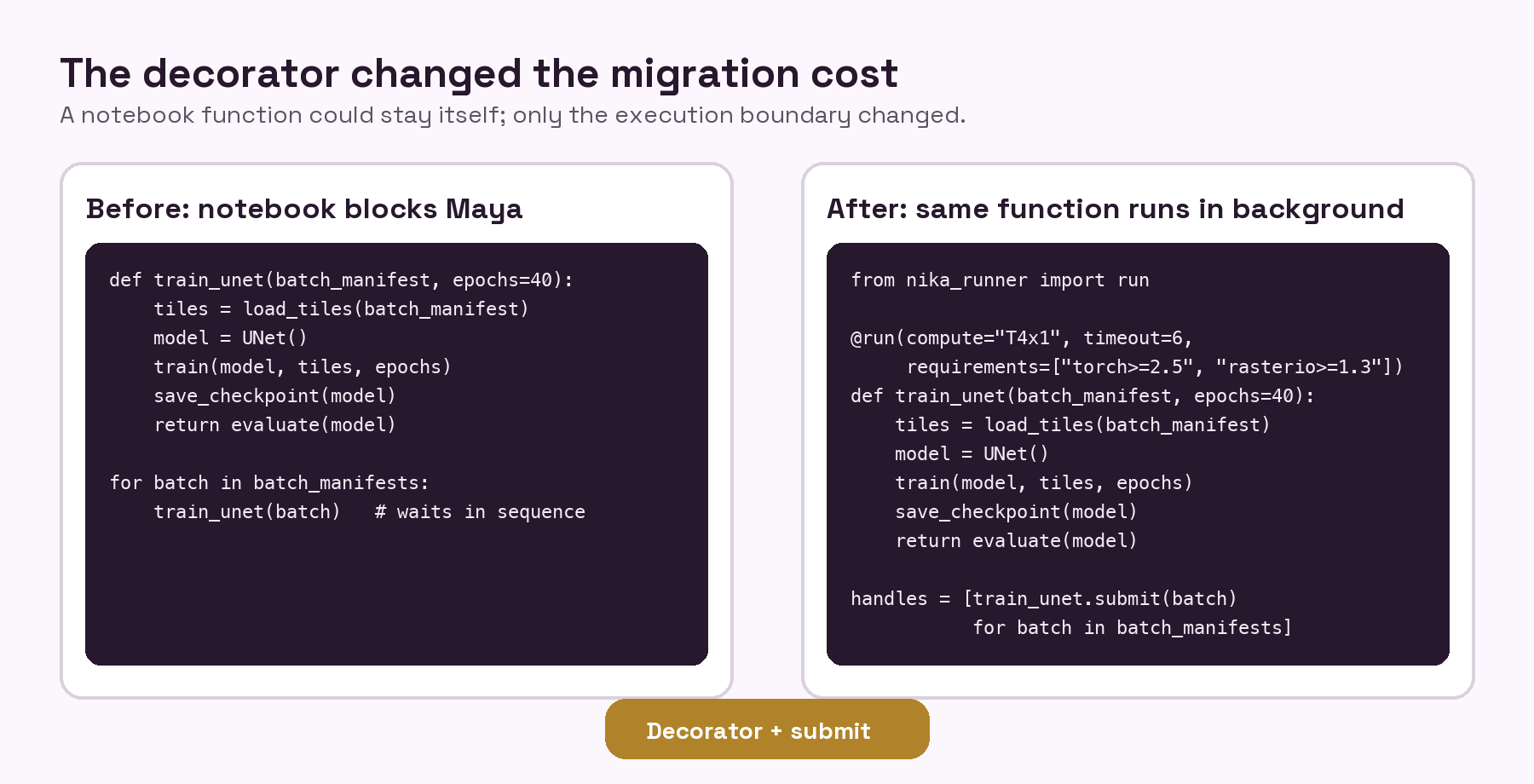
Code comparison: the Python function stays recognizable; the decorator tells NIKA Runner where and how to execute it.
Once the first notebook worked, the pattern spread. The U-Net training function became a T4 job. The chip-building function moved to CPU because it was mostly raster and vector preprocessing. The ViT experiment used a bigger GPU only when the model deserved it. Maya was no longer converting a project all at once. She was moving one expensive function at a time into the background, then watching the runs from the workspace.
The next layer was operational rather than syntactic: list_runs() to see the queue, load_run() to reopen a result, logs for debugging, child runs for fan-out work, and cancellation when an experiment was clearly wrong. Those details mattered because she was not trying to write a demo. She was trying to keep ten imperfect notebooks moving toward one delivery deadline.
The UI changed the budget conversation
The biggest change was not that the jobs ran. It was that she could see them. The NIKA Runner UI showed active runs, completed runs, failed runs, child runs, logs, and the machine attached to each job. The usage graphs for CPU, GPU, and RAM turned compute from a black box into a planning tool. If preprocessing barely touched the GPU, it moved to CPU. If a model saturated memory before compute, she changed the machine. If a small batch ran no faster on premium hardware, she stopped spending premium credits there.
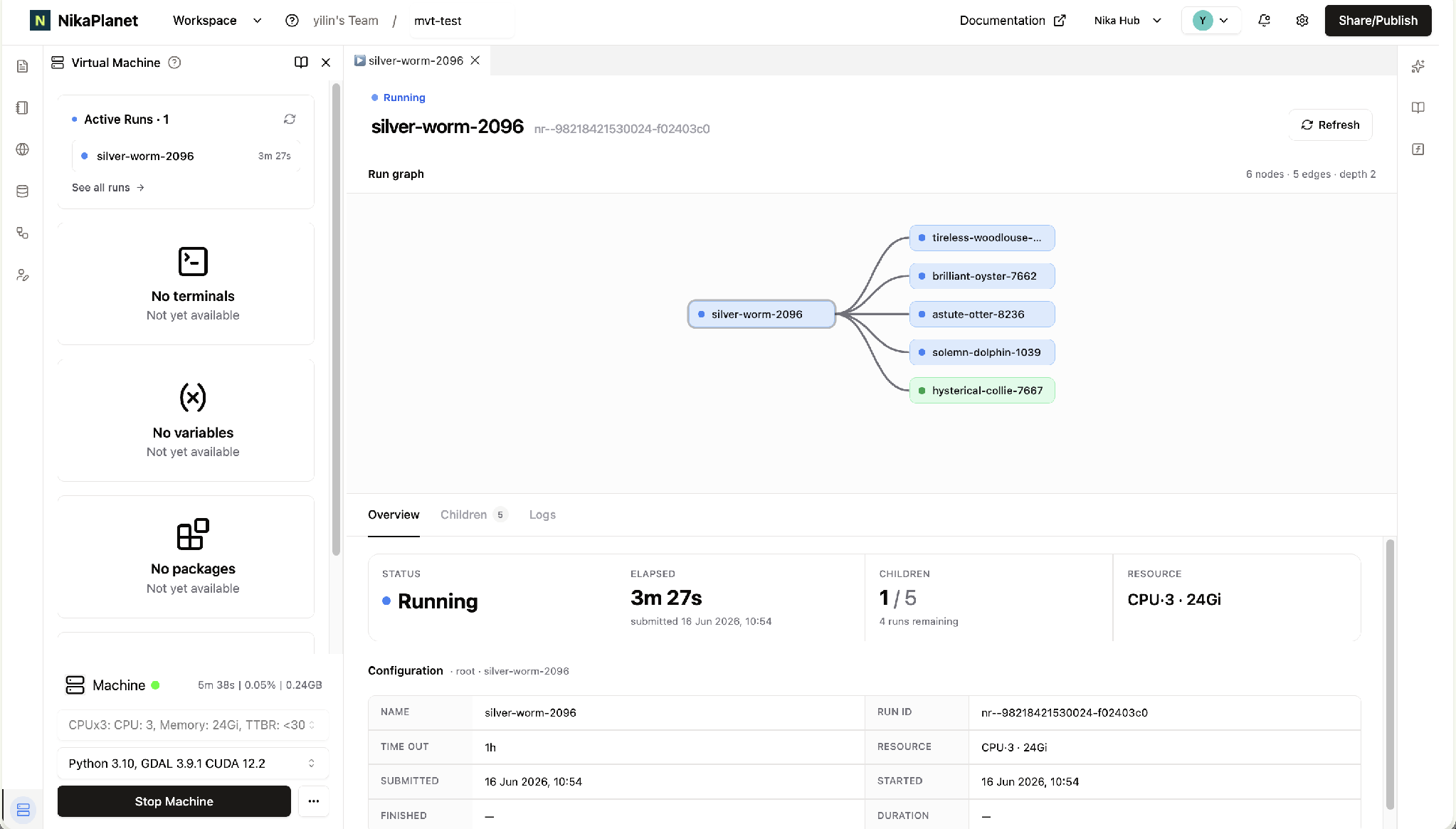
Figure: NIKA Runner UI for monitoring active, historical, and fan-out geospatial compute jobs.
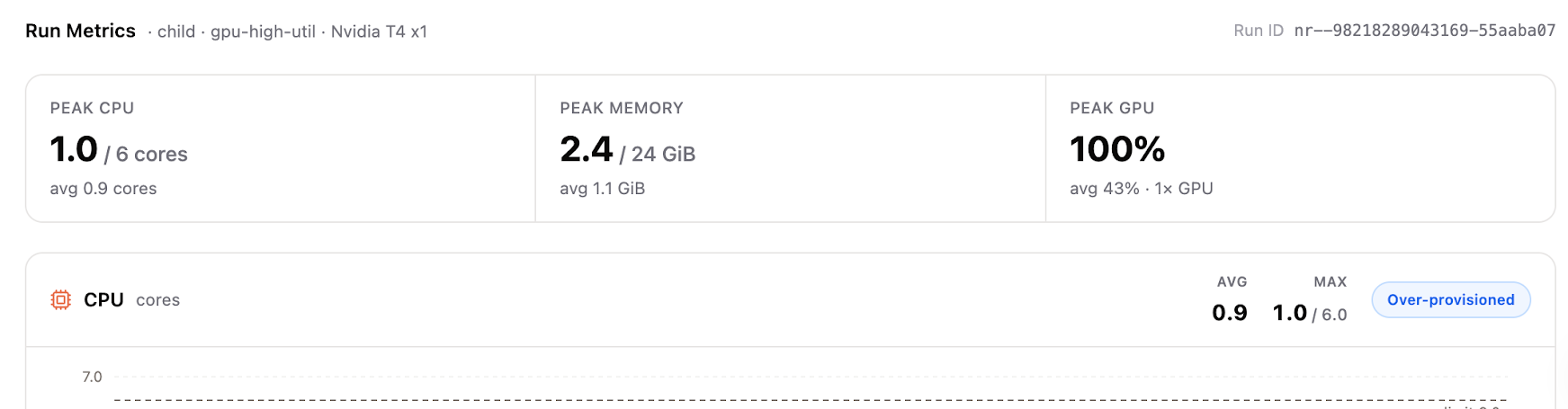
Figure: Run metrics summarize CPU, memory, and GPU peaks so the team can spot over-provisioned jobs.
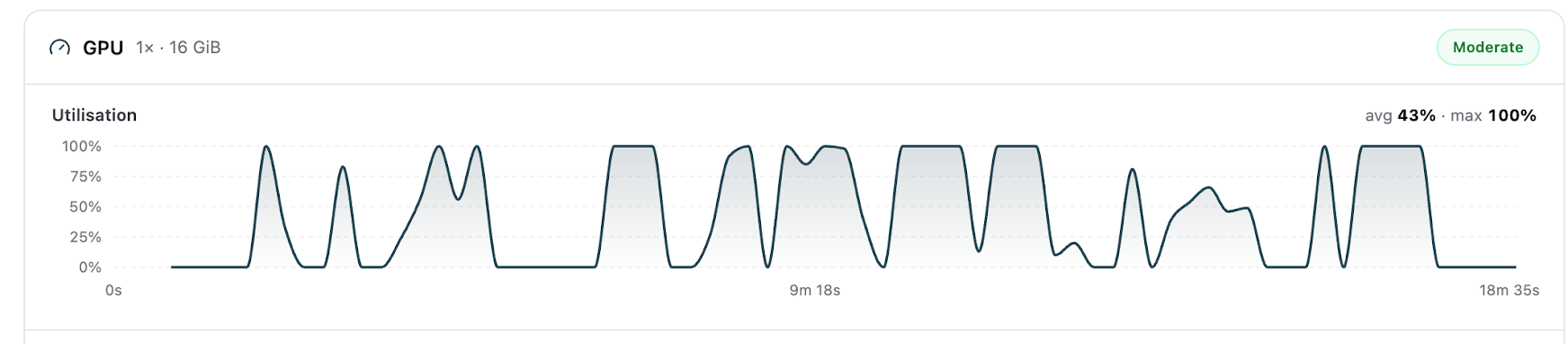
Figure: GPU utilization over time shows whether a training job is actually using the machine it requested.
The larger platform discovery
As Maya used NIKA Runner SDK, she realised NikaPlanet isn't just the launchpad for computation jobs; NikaPlanet is the entire space station. The team could keep datasets in one workspace, open notebooks against the same storage, visualize outputs on maps, and work toward a loop where imagery, labeling, training, inference, and review lived closer together.
She also found NIKA Labeler, the annotation tool on the same platform. That mattered because agriculture ML is only as good as the masks and labels feeding it. A better label workflow meant the next model iteration would start upstream, before training. Testing NIKA Labeler properly would become a separate story, but even seeing it there changed how she thought about the project. The compute layer was not alone; it belonged to a platform for geospatial teams.
What changed by the end of the month
The task did not suddenly become easy - nothing does. However, the key was that it became surmountable. Instead of one slow lane, Maya had parallel tracks: CPU jobs prepared tiles while T4 jobs trained and H100-class runs handled the experiments that deserved them. The team could compare outputs with time left to improve labels and rerun weak batches. The same amount of work no longer had to happen in the same order.
The project that she could barely have met in a sequential workflow became something she could deliver with breathing room. The difference was not magic. It was parallelism, right-sized machines, shared storage, and a UI that made the invisible parts of compute visible.
The story of more than just Maya
These problems are not unique to Maya. Teams building on geospatial Python run into the same walls: the analyst who does not want to repackage GDAL for the third time, the ML lead trying to spend GPU credits carefully, the team that needs logs and child runs visible without spinning up an entire DevOps practice to get there. We have been listening to that pattern across many clients. NIKA is designed and built alongside those complaints — not as another generic cloud compute layer, but as a workbench that lets massive geospatial Python workloads scale without pulling the scientist away from the science. The portal to read more about NIKA Runner SDK is right here to get you started.